Tutorials¶

1. Basic active space selection¶

In this section we go step by step through simple examples, highlighting the output of the code, in order to introduce the user to the basic concepts behind the ASF software. All input files are available in the example folder of the package.

1.1. Selecting an active space for ethene¶

As an introductory example, we will demonstrate the selection of an active space for ethene (\(\text{C}_2\text{H}_4\)). While the ground state does not have a strongly correlated wave function, it is suited to illustrate the basic ideas. The input for the calculation is in the file examples/ethene/c2h4.py. Here, we will examine the input step by step.

Start by importing the required functionality of PySCF and the ASF:

from pyscf import gto, mcscf
from pyscf.lib import logger

from asf.wrapper import runasf_from_mole
from asf.utility import pictures_Jmol

Next, we specify the molecule by instantiating a PySCF Mole object. The atomic positions are contained in the file examples/ethene/c2h4.xyz in the same directory.

# Set up the molecule.
mol = gto.Mole()
mol.atom = 'c2h4.xyz'
mol.basis = 'def2-SVP'
mol.spin = 0
mol.charge = 0
mol.verbose = logger.INFO
mol.build()

Having set up the molecule, we pass it on to the “all-in-one” wrapper function, which also performs the SCF calculation:

# Wrapper function to:
#
# 1) Perform an SCF calculation
# 2) Calculate MP2 natural orbitals.
# 3) Run CASCI in a subset of MP2 natural orbitals.
# 4) Perform the orbital selection.
#
# We get:
# nel:      Number of electrons in the selected active space.
# mo_list:  List of orbitals making up the active space.
# mo_coeff: The matrix containing the MO coefficients (active and inactive).
#           Here, the MO coefficients are MP2 natural orbitals. The rows of the matrix index AOs,
#           the columns index MOs.
nel, mo_list, mo_coeff = runasf_from_mole(mol)

The wrapper function performs an unrestricted Hartree-Fock (UHF) calculation first. Even if the electronic state is a singlet, for strongly correlated molecules the UHF will typically undergo a symmetry breaking, leading to a spin-contaminated wave function. This is done here on purpose.

A stability analysis is performed; even for ethene, it is possible to lower the energy by introducing a small amount of spin contamination.

converged SCF energy = -77.9774983467955  <S^2> = 3.0890863e-09  2S+1 = 1

Performing stability analysis.
UHF/UKS wavefunction has an internal instability.

SCF solution unstable.
Restarting the SCF calculation.

The first solution is unstable, which triggers a new SCF calculation:

converged SCF energy = -77.977530565129  <S^2> = 0.032286977  2S+1 = 1.0626137

Performing stability analysis.
UHF/UKS wavefunction is stable in the internal stability analysis

-> SCF solution converged and stable.

In more complicated cases, it may be preferable to set up and run the Hartree-Fock calculation manually. In that case, the SCF object would be passed to the function asf.wrapper.runasf_from_scf.

Having an SCF solution, a smaller orbital space needs to be found to perform a DMRG calculation. While it would be possible to just select a window of Hartree-Fock orbitals based on their energy, this is not generally a good approach to select active spaces. We made better experiences with MP2 natural orbitals (which are calculated from an unrelaxed density, and have got associated natural occupation numbers between two and zero). Please note that the active space is selected from MP2 natural orbitals, not from SCF orbitals! When calling runasf_from_scf(mf, ...) with an SCF object mf, the list of active orbitals returned by the function does not refer to the matrix mf.mo_coeff. The active orbital list always refers to the MO coefficients, consisting of MP2 natural orbitals, that are returned by runasf_from_mole and runasf_from_scf.

--------------------------------------------------------------------------------
Calculating MP2 natural orbitals
--------------------------------------------------------------------------------

[...]

-> Selected initial orbital window of 12 electrons in 12 MP2 natural orbitals.

A special remark needs to be made regarding the MP2 implementation. PySCF 1.7.6 only has a conventional implementation of MP2 for UHF references, which may become unfeasible for larger systems. HQS contributed a more efficient DF-MP2 implementation to PySCF, which has been released in version 2 of PySCF. The ASF code attempts to use the latter if it is available. Since the current version of the ASF is based on PySCF 1.7.6, using the more efficient DF-MP2 implementation is somewhat tricky, and requires patching the code. The most convenient way to install a patched PySCF together with Block is to use the build script build_script/PySCF_Block.sh provided with ASF.

Having selected a subset of MP2 natural orbitals, these are normally used for a DMRG calculation. However, if the number of orbitals is sufficiently small, the code performs a normal CASCI calculation, instead. Based on the calculated entropies, an active space is selected:

Orbital selection for state 0:

MO    w( )    w(↑)    w(↓)    w(⇅)       S  sel
 0.001   0.006   0.006   0.987   0.079
 0.002   0.007   0.007   0.984   0.099
 0.003   0.007   0.007   0.983   0.105
 0.004   0.007   0.007   0.982   0.107
 0.004   0.009   0.009   0.979   0.125
 0.029   0.008   0.008   0.954   0.226    a
 0.954   0.008   0.008   0.030   0.228    a
 0.984   0.007   0.007   0.003   0.101
 0.984   0.006   0.006   0.004   0.102
 0.984   0.007   0.007   0.002   0.098
 0.982   0.007   0.007   0.003   0.106
 0.983   0.007   0.007   0.003   0.102

The first column contains the orbital index (counting starts from zero). Columns two to five show the probability for each spatial orbital to have an occupation out of the four possibilities empty, spin-up, spin-down or doubly occupied. The sixth column contains the one-orbital entropy. Finally, a flag in the seventh column indicates whether an orbital has been selected for the active space.

We can create image files of the orbitals for visual inspection:

# Plot the orbitals.
pictures_Jmol(mol, mo_coeff, mo_list=mo_list, rotate=(-45, 0, 0))

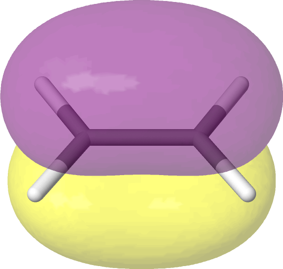
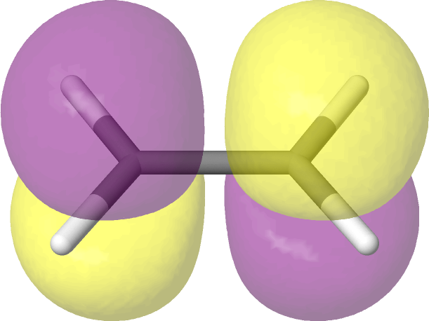
As expected, the ASF selects an active space consisting of the HOMO and LUMO of ethane. Note that Jmol (the software used to create the images) labels orbitals starting from one, not from zero. The default entropy cutoff for orbital selection in the ASF wrapper functions runasf_from_[...] can be modified with the entropy_threshold keyword option, e.g. runasf_from_mole(..., entropy_threshold=0.2).

Having selected an active space, we are in a position to perform a CASSCF or CASCI calculation:

# Now we set up a CASSCF calculation.
# ncas: number of active orbitals
ncas = len(mo_list)
mc = mcscf.CASSCF(mol, ncas, nel)

# Generally, we need to sort the MOs such that the columns are ordered from left to right:
# 1) occupied inactive
# 2) active
# 3) unoccupied inactive
# Note that python counts from 0 by default, but the default value for base in sort_mo is 1.
# Therefore, we need to set base=0 explicitly.
mo_sorted = mc.sort_mo(mo_list, mo_coeff=mo_coeff, base=0)

# Run the CASSCF calculation.
mc.kernel(mo_coeff=mo_sorted)

Note that it is important to reorder the columns of the MO coefficients before passing them to a CAS object.

The wrapper functions have an option sort_mos. If it is set to True, the reordering is performed within the wrapper:

nel, mo_list, mo_coeff = runasf_from_mole(mol, sort_mos=True)
mc = mcscf.CASSCF(mol, len(mo_list), nel)
mc.kernel(mo_coeff=mo_coeff)

In this case, however, the table with the entropies printed by the wrapper still refers to the original ordering of the orbitals used internally during the selection; it is not consistent with the columns in the mo_coeff returned.

1.2 Vertical excitation energies in benzene¶

In the previous example, we showed how the ASF can be used to select an active space for a CASSCF calculation. Here, we go one step further by demonstrating that an automatically chosen active space for benzene leads to identical results as a manually selected one. We proceed to calculate the vertical excitation energy between the lowest two singlet states of benzene, and compare it to the experimental result from vacuum ultraviolet (VUV) spectra.

In this example, we use the wrapper function that is called with a converged Hartree-Fock object.

from pyscf import gto, scf, mcscf, mrpt
from pyscf.data.nist import HARTREE2EV

from asf.wrapper import runasf_from_scf
from asf.utility import pictures_Jmol

To this end, we start by initializing the Mole object, and perform the mean-field calculation manually.

###################################################################################################
# Molecule setup and RHF calculation.
###################################################################################################
mol = gto.Mole()
mol.atom = 'benzene.xyz'
mol.basis = 'def2-tzvp'
mol.verbose = 4
mol.max_memory = 2500
mol.build()

mf = scf.RHF(mol).density_fit()
mf.kernel()

The geometry is stored in the file examples/benzene/benzene.xyz. Now, we can call the wrapper function to perform the active space selection procedure.

# Get active space of first two singlet states
act_el, act_mos, natorbs = runasf_from_scf(mf, mp2_kwargs={'max_orb': 15}, states=2)

Here, the wrapper function is called with the arguments states and mp2_kwargs. In this case, states is specified as an integer \(n\): this tells the wrapper to perform the active space selection for the \(n\) lowest states of the same spin multiplicity as specified in the Mole object. Alternatively, states can be defined as a list of tuples [(s1, n1), (s2, n2), ...]. In that case, the wrapper performs the active space selection for n1 states of spin s1, n2 states of spin s2, etc. For example, [(0, 2), (2, 1)] means to perform the calculation for two singlet states and one triplet state. The active spaces determined for all individual electronic states are merged in the return value of the wrapper. We follow the convention of PySCF to define “spin” option as the “number of unpaired electrons”.

mp2_kwargs can be used to pass a dictionary of keyword arguments to the function that performs an initial orbital selection from MP2 natural orbitals. Here, we have used a low cutoff max_orb to limit the number of orbitals in the DMRG calculation to 15. In general, however, it is advisable to use a larger initial orbital set.

Except for the SCF calculation, the wrapper function follows the same procedure as before, starting with an MP2 calculation to select an initial active space.

--------------------------------------------------------------------------------
Calculating MP2 natural orbitals
--------------------------------------------------------------------------------

[...]

-> Selected initial orbital window of 14 electrons in 15 MP2 natural orbitals.

Next, DMRG-CI calculations are performed for the two lowest singlet states.

spin = 0, number of roots = 2

[...]

CASCI state 0  E = -230.90948786347  E(CI) = -33.9742774171603  S^2 = 0.0000000
CASCI state 1  E = -230.675148878741  E(CI) = -33.7399384324316  S^2 = 0.0000000
Orbital selection for state 0:

MO    w( )    w(↑)    w(↓)    w(⇅)       S  sel
 0.001   0.003   0.003   0.993   0.046
 0.002   0.007   0.007   0.985   0.090
 0.001   0.005   0.005   0.989   0.073
 0.001   0.005   0.005   0.989   0.073
 0.004   0.012   0.012   0.972   0.158    a
 0.017   0.018   0.018   0.946   0.269    a
 0.016   0.019   0.019   0.945   0.271    a
 0.945   0.019   0.019   0.017   0.275    a
 0.945   0.019   0.019   0.018   0.274    a
 0.974   0.012   0.012   0.003   0.147    a
 0.988   0.005   0.005   0.001   0.076
 0.988   0.005   0.005   0.001   0.077
 0.991   0.004   0.004   0.001   0.061
 0.993   0.003   0.003   0.001   0.051
 0.997   0.001   0.001   0.001   0.025

Orbital selection for state 1:

MO    w( )    w(↑)    w(↓)    w(⇅)       S  sel
 0.001   0.002   0.002   0.994   0.041
 0.002   0.006   0.006   0.986   0.088
 0.001   0.005   0.005   0.990   0.068
 0.001   0.005   0.005   0.990   0.068
 0.010   0.043   0.043   0.904   0.408    a
 0.022   0.248   0.248   0.482   1.127    a
 0.022   0.250   0.250   0.478   1.130    a
 0.477   0.248   0.248   0.027   1.143    a
 0.472   0.250   0.250   0.028   1.147    a
 0.923   0.035   0.035   0.007   0.345    a
 0.990   0.005   0.005   0.001   0.068
 0.990   0.005   0.005   0.001   0.068
 0.991   0.004   0.004   0.001   0.057
 0.993   0.003   0.003   0.001   0.049
 0.996   0.001   0.001   0.001   0.027

--------------------------------------------------------------------------------
Active space selection finished
--------------------------------------------------------------------------------

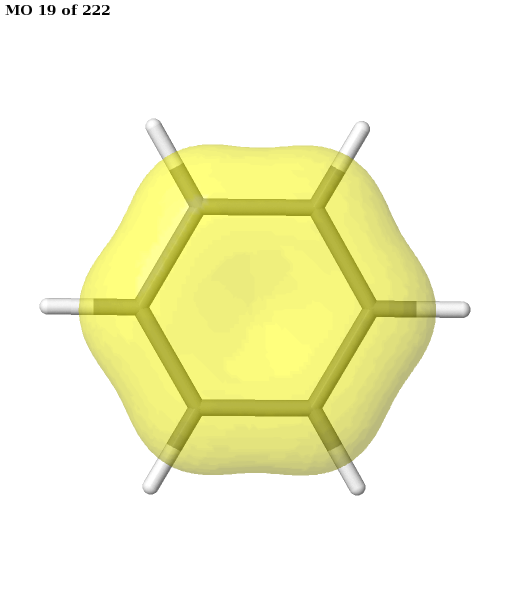
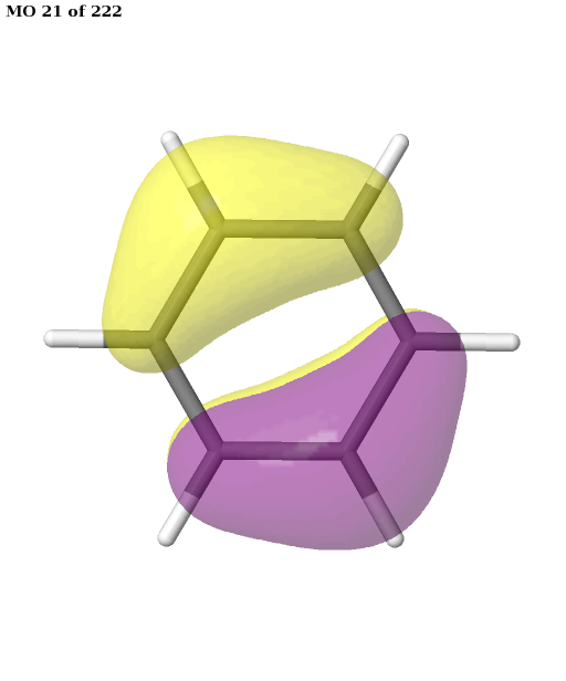
-> Selected an active space of 6 electrons in 6 orbitals.

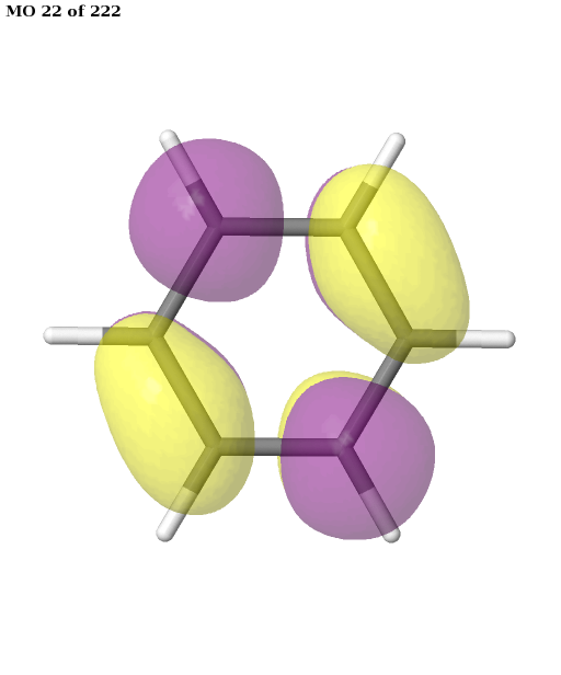
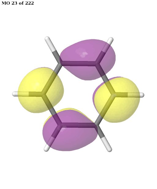
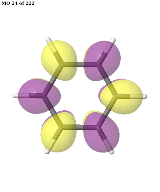
The final active space is a union of the orbital sets selected for each root (electronic state). It contains six electrons in six orbitals: the \(\pi\) and \(\pi^{\star}\) orbitals of benzene. This is a common choice for the active space, which is used, for example, in this publication. We can plot these orbitals as shown in the previous example (keep in mind that Jmol starts counting the molecular orbitals from 1).

# plot orbitals
pictures_Jmol(mol, natorbs, act_mos, rotate=(90, 0, 0))

Having selected the active space based on ground- and excited-state calculations, we carry out a state-average CASSCF calculation, which optimizes a single set of orbitals for a weighted average of the energies for both states.

Note

Since we are interested in calculating the excited state with the same spin and symmetry, we employ state-averaged CASSCF. Note that state-averaged CASSCF should be performed with equal weights for all states, as using a higher ensemble weight for an excited state can cause convergence issues, for example a flipped energetical ordering of the states.

# CASSCF with ASF orbitals
# State average CASSCF.
mcASF = mcscf.CASSCF(mf, len(act_mos), act_el).state_average_(weights=(0.5, 0.5))
mcASF.fix_spin()
mo_sorted = mcASF.sort_mo(act_mos, mo_coeff=natorbs, base=0)
mcASF.kernel(mo_coeff=mo_sorted)

For comparison with experimental results, we perform a NEVPT2 calculation to include dynamic correlation on top of the CASSCF results. Since this cannot be done directly with the state-average CASSCF objects, we need to first perform a CASCI calculation with the converged orbitals, first.

# Now, we calculate the NEVPT2 energies of the two electronic states.
# Since NEVPT2 cannot work with state-averaged CASSCF objects, we need to set up a CASCI object.
mciASF = mcscf.CASCI(mf, len(act_mos), act_el)
mciASF.fcisolver.nroots = 2
mciASF.fix_spin()
# Calculate the CASCI energies
e1 = mciASF.kernel(mo_coeff=mcASF.mo_coeff)
# Calculate the NEVPT2 correlation energies for both roots separately.
e_corrASF0 = mrpt.NEVPT(mciASF, root=0).kernel()
e_corrASF1 = mrpt.NEVPT(mciASF, root=1).kernel()

We can repeat the calculation by selecting a set of RHF orbitals manually. Since we also select a set of \(\pi\) orbitals, the CASSCF calculation converges to the same result:

# The hand-picked (6, 6) active space with canonical RHF orbitals.
orb_manual = [16, 19, 20, 21, 22, 30]
# State average CASSCF.
mc_manual = mcscf.CASSCF(mf, len(orb_manual), act_el).state_average_(weights=(0.5, 0.5))
mc_manual.fix_spin()
mo_sorted = mc_manual.sort_mo(orb_manual, mo_coeff=mf.mo_coeff, base=0)
mc_manual.kernel(mo_coeff=mo_sorted)

As before, the NEVPT2 energy is calculated with the converged state-averaged CASSCF orbitals.

# Calculate the NEVPT2 energies of the two electronic states.
# As before, we need to set up a new CASCI object.
mci_manual = mcscf.CASCI(mf, len(orb_manual), act_el)
mci_manual.fcisolver.nroots = 2
mci_manual.fix_spin()
# Calculate the CASCI energies.
e2 = mci_manual.kernel(mo_coeff=mc_manual.mo_coeff)
# Calculate the NEVPT2 correlation energies for both roots separately.
e_corr_man0 = mrpt.NEVPT(mci_manual, root=0).kernel()
e_corr_man1 = mrpt.NEVPT(mci_manual, root=1).kernel()

Finally we calculate the excitation energies and print the results.

CAS_ex = (e1[0][1] - e1[0][0]) * HARTREE2EV
PT_ex = CAS_ex + (e_corrASF1 - e_corrASF0) * HARTREE2EV
print('CASSCF excitation energy with automatic selection: {0:.3f} eV'.format(CAS_ex))
print('NEVPT2 excitation energy with automatic selection: {0:.3f} eV'.format(PT_ex))
CAS_ex = (e2[0][1] - e2[0][0]) * HARTREE2EV
PT_ex = CAS_ex + (e_corr_man1 - e_corr_man0) * HARTREE2EV
print('CASSCF excitation energy with manual selection: {0:.3f} eV'.format(CAS_ex))
print('NEVPT2 excitation energy with manual selection: {0:.3f} eV'.format(PT_ex))

CASSCF excitation energy with automatic selection: 5.000 eV
NEVPT2 excitation energy with automatic selection: 5.379 eV
CASSCF excitation energy with manual selection: 5.000 eV
NEVPT2 excitation energy with manual selection: 5.379 eV

The calculations with the automatically and manually selected active spaces yield the same result. Experimental values for this excitation energy are around 4.9 eV (for instance 4.86 eV). More accurate calculations using NEVPT2/def2-TZVP are possible by selecting a much larger active space to include a larger fraction of dynamic correlation in the CASSCF calculation.

The script for this example can be found under examples/benzene/benzene.py.

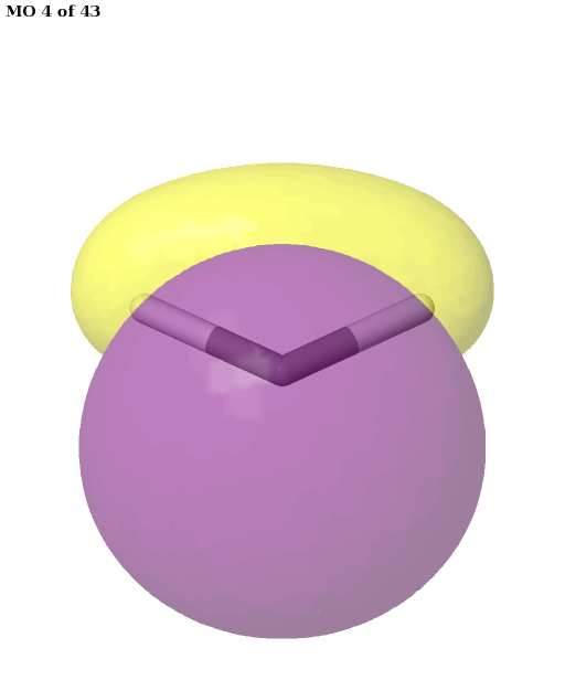
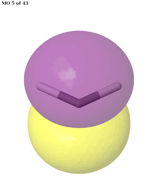
1.3 Using wrapper function to select an active space for methylene¶

In this example, we will calculate the singlet-triplet splitting for methylene (\(\mathrm{CH}_2\)). \(\mathrm{CH}_2\) is an organic molecule with a triplet ground state, which appears as an intermediate in some chemical reactions. This system has two nearly-degenerate orbitals, MO 3 and MO 4 (counting starts from zero), which are shown below. For the singlet spin state, this leads to a wave function with some multi-reference character. Note that the indices in Jmol plots are shifted by one compared to the PySCF indexing, as jmol starts counting the molecular orbitals from 1.

We start by importing relevant functionality:

from pyscf import gto, mcscf
from asf.wrapper import runasf_from_mole
from asf.utility import pictures_Jmol

The molecular geometry, the spin multiplicity and the basis set basis for the molecule are set in an instance of the PySCF Mole object. The coordinates are imported from file examples/methylene/ch2.xyz

# build the mol object
mol = gto.Mole()
mol.atom = 'ch2.xyz'
mol.basis = 'def2-tzvp'
mol.spin = 2
mol.verbose = 4
mol.max_memory = 2500
mol.build()

In this case, we have set the spin state to a triplet: the reason is that the Hartree-Fock calculation is easier to converge than for the singlet, where SCF instabilities and multiple minima are more likely to be encountered.

Now, we hand the molecule object directly over to the wrapper function.

# Get active space of first two singlet states
nel, mo_list, mo_coeff = runasf_from_mole(mol, states=[(0, 1), (2, 1)], entropy_threshold=0.2,
                                          switch_dmrg=4)

The following options are provided to the wrapper function:

states=[(0, 1), (2, 1)] In each tuple within the list, the first integer indicates the spin state (through the number of unpaired electrons), and the second integer specifies the number of roots to be calculated for that state. Here, we include one singlet and one triplet state. Entropies are calculated for each state independently, but the resulting active space is the union of all sets of active orbitals determined independently.
entropy_threshold = 0.2 We change the entropy threshold from the default value (see below).
switch_dmrg = 4 The wrapper only enables DMRG if the number of orbitals is above a threshold, which has a value of 12 by default. Below this threshold, the entropies are calculated using a normal CI algorithm instead of DMRG. Here, we show how this threshold can be modified. Beware: if you remove this option, and use the default CI algorithm of PySCF in this example, it is prone to converge to an excited state.

Inside the wrapper function, a UHF calculation is performed for the triplet state, as specified in the Mole object:

--------------------------------------------------------------------------------
Calculating UHF orbitals
--------------------------------------------------------------------------------

[...]

converged SCF energy = -38.9328376672972  <S^2> = 2.0128193  2S+1 = 3.0085341

Performing stability analysis.
UHF/UKS wavefunction is stable in the internal stability analysis

-> SCF solution converged and stable.

The UHF reference is used to calculate MP2 natural orbitals, from which an initial orbital window is selected:

--------------------------------------------------------------------------------
Calculating MP2 natural orbitals
--------------------------------------------------------------------------------

[...]

-> Selected initial orbital window of 8 electrons in 10 MP2 natural orbitals.

After performing the CI calculation, the following entropies and occupancies are obtained for the singlet state:

MO    w( )    w(↑)    w(↓)    w(⇅)       S  sel
 0.000   0.000   0.000   1.000   0.001
 0.006   0.006   0.006   0.983   0.105
 0.008   0.006   0.006   0.980   0.121
 0.059   0.007   0.007   0.928   0.301    a
 0.939   0.001   0.001   0.059   0.240    a
 0.984   0.005   0.005   0.005   0.101
 0.986   0.004   0.004   0.005   0.088
 0.990   0.004   0.004   0.001   0.067
 0.995   0.002   0.002   0.001   0.037
 0.998   0.001   0.001   0.000   0.017

We see immediately that MOs 3 and 4 are the most strongly entangled ones.

The wrapper also calculates occupations and entropies for the triplet state, which are shown in the following table:

MO    w( )    w(↑)    w(↓)    w(⇅)       S  sel
 0.000   0.000   0.000   1.000   0.001
 0.004   0.011   0.005   0.980   0.119
 0.008   0.008   0.008   0.976   0.139
 0.004   0.992   0.001   0.003   0.053    a
 0.005   0.991   0.003   0.000   0.057    a
 0.982   0.008   0.005   0.005   0.110
 0.983   0.007   0.005   0.005   0.104
 0.994   0.003   0.001   0.001   0.041
 0.996   0.002   0.001   0.001   0.029
 0.994   0.006   0.000   0.000   0.037

As the MOs 3 and 4 are singly occupied, they need to be included in the active space. With the default entropy cutoff of 0.139, MO 2 would just about have been selected for the active space, too. Since we wanted to obtain the minimal (2, 2) active space of two electrons in two orbitals, we have adjusted the selection threshold accordingly. The wrapper function merges the sets of active orbitals that have been determined for each state (and which are identical in this case).

The selected orbitals can be plotted using Jmol. We have adapted the mo_list option to create images of all valence orbitals. rotate controls the orientation of the molecule in the plots by rotating it around the x-, y- and z-axes.

# plot the valence orbitals
pictures_Jmol(mol, mo_coeff, mo_list=[1, 2, 3, 4, 5, 6], rotate=(45, 0, 0))

Finally, we can use the generated orbitals, with the selected active space, for CASSCF. Here, we perform two independent CASSCF calculations for the singlet and the triplet states. The energy gap between the singlet and triplet states can be obtained by subtracting the respective energy values.

# CASSCF with ASF orbitals for the singlet and the triplet
for spin in 0, 2:
    print('\nCASSCF with spin = {0:d}\n'.format(spin))
    mc = mcscf.CASSCF(mol, len(mo_list), nel)
    mc.fcisolver.spin = spin
    mc.fix_spin()
    mo_sorted = mc.sort_mo(mo_list, mo_coeff=mo_coeff, base=0)
    mc.kernel(mo_coeff=mo_sorted)

Of course, it is also possible to perform a state-averaged calculation for both spin states; or to include dynamic correlation via a method such as NEVPT2.

The script for this example can be found under examples/methylene/CH2.py.

2 Transition metal system: hexaaqua iron III¶

The hexaaqua iron (III) complex, \([\text{Fe}(\text{H}_2\text{O})_6]^{3+}\), possesses a sextet ground state. By undergoing a spin-forbidden d-d transition, the complex can be excited into a quartet state; the three lowest quartet states are near-degenerate.

In the example file example/hexaaqua_iron_iii/complex.py, we demonstrate how an active space selection can be performed for the aforementioned electronic states. The script starts with a UHF calculation for the sextet ground state, which is passed on to the ASF wrapper after convergence. In order to reduce the computational expense for this example, the number of MP2 natural orbitals is limited to 15:

# Use the ASF for lowest quartet and sextet states.
states = [(5, 1), (3, 3)]
act_ele, act_mos, mp2orb = runasf_from_scf(mf, mp2_kwargs={'max_orb': 15}, states=states, maxM=150)

The subsequent DMRG calculations to select an active space are performed for one sextet and the three quartet states separately.

For the sextet, the following occupations and entropies are obtained:

MO    w( )    w(↑)    w(↓)    w(⇅)       S  sel
 0.000   0.001   0.001   0.998   0.013
 0.000   0.001   0.000   0.999   0.012
 0.000   0.000   0.000   0.999   0.010
 0.000   0.001   0.001   0.998   0.014
 0.000   0.001   0.001   0.998   0.014
 0.000   0.999   0.000   0.001   0.006    a
 0.000   0.999   0.000   0.001   0.006    a
 0.000   1.000   0.000   0.000   0.000    a
 0.000   1.000   0.000   0.000   0.000    a
 0.000   1.000   0.000   0.000   0.000    a
 0.997   0.001   0.001   0.001   0.022
 0.999   0.000   0.000   0.000   0.009
 0.999   0.000   0.000   0.000   0.010
 0.999   0.000   0.000   0.000   0.010
 0.999   0.000   0.000   0.000   0.005

The entropies are so low, because the small subset of 15 MP2 natural orbitals does not include appropriate correlation partners. For example, the partner orbitals of the 3d shell of Fe are its 4d orbitals. Only the five singly occupied orbitals are selected to represent the active space.

Next, we inspect the results for the three quartet states:

Orbital selection for state 0:

MO    w( )    w(↑)    w(↓)    w(⇅)       S  sel
 0.000   0.001   0.001   0.998   0.014
 0.000   0.001   0.001   0.998   0.013
 0.000   0.000   0.000   0.999   0.010
 0.001   0.002   0.006   0.990   0.063
 0.000   0.002   0.001   0.997   0.025
 0.047   0.950   0.000   0.003   0.212    a
 0.896   0.077   0.001   0.027   0.397    a
 0.011   0.979   0.000   0.010   0.120    a
 0.010   0.979   0.000   0.011   0.120    a
 0.027   0.021   0.000   0.952   0.225    a
 0.997   0.001   0.001   0.001   0.023
 0.999   0.000   0.000   0.000   0.009
 0.999   0.000   0.000   0.000   0.010
 0.999   0.000   0.001   0.000   0.011
 0.999   0.000   0.000   0.000   0.006

Orbital selection for state 1:

MO    w( )    w(↑)    w(↓)    w(⇅)       S  sel
 0.000   0.001   0.001   0.998   0.014
 0.000   0.001   0.001   0.998   0.013
 0.000   0.000   0.000   0.999   0.011
 0.000   0.002   0.001   0.997   0.023
 0.001   0.002   0.006   0.990   0.064
 0.860   0.114   0.001   0.025   0.475    a
 0.083   0.913   0.000   0.004   0.314    a
 0.027   0.021   0.000   0.952   0.225    a
 0.011   0.979   0.000   0.010   0.120    a
 0.010   0.979   0.000   0.011   0.120    a
 0.997   0.001   0.001   0.001   0.023
 0.999   0.000   0.000   0.000   0.010
 0.999   0.000   0.000   0.000   0.010
 0.999   0.000   0.000   0.000   0.010
 0.999   0.000   0.000   0.000   0.006

Orbital selection for state 2:

MO    w( )    w(↑)    w(↓)    w(⇅)       S  sel
 0.000   0.001   0.001   0.998   0.014
 0.000   0.001   0.000   0.999   0.012
 0.000   0.000   0.000   0.999   0.011
 0.001   0.002   0.004   0.993   0.046
 0.001   0.002   0.003   0.994   0.043
 0.507   0.476   0.001   0.016   0.767    a
 0.436   0.550   0.001   0.013   0.753    a
 0.010   0.979   0.000   0.011   0.120    a
 0.027   0.021   0.000   0.952   0.225    a
 0.011   0.979   0.000   0.010   0.120    a
 0.997   0.001   0.001   0.001   0.023
 0.999   0.000   0.000   0.000   0.009
 0.999   0.000   0.000   0.000   0.010
 0.999   0.001   0.000   0.000   0.010
 0.999   0.000   0.000   0.000   0.005

Here, the orbitals are more strongly entangled. In each case, the ASF selects a minimal active space consisting of the five 3d orbitals, which are shown below.

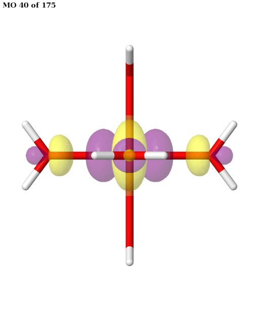
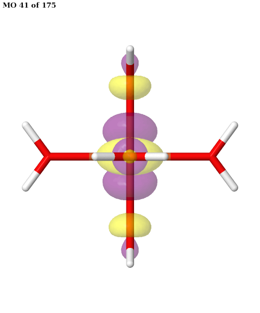
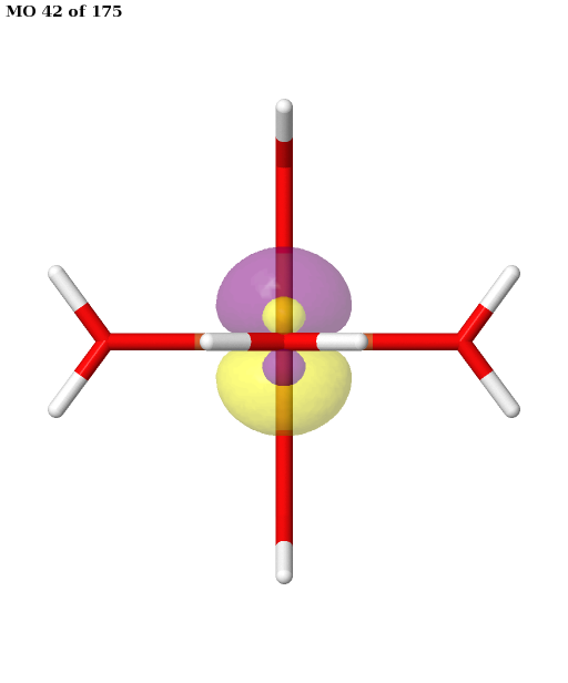
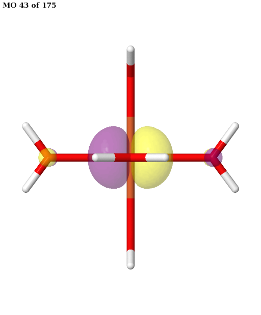
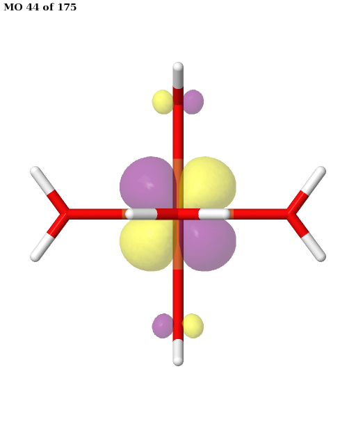
Finally, the selected active space is used in a state-averaged CASSCF calculation. We use a weight of \(1/2\) for the sextet, and a total weight of \(1/2\) for the quartet, or \(1/6\) for each of the three near-degenerate quartet states.

# We want to perform a state-averaged CASSCF calculation, which includes the sextet ground state
# and three triplet states.
# First define the full-CI solvers for the diffecent spin states.
# Sextet
solver5 = fci.FCI(mol)
solver5.spin = 5
solver5.nroots = 1
# Quartet: we want to calculate three states
solver3 = fci.FCI(mol)
solver3.spin = 3
solver3.nroots = 3
# Ensure the the spin does not change
solvers = [fci.addons.fix_spin(s) for s in (solver5, solver3)]

# We use the MP2 natural orbitals that are returned by the wrapper function.
cas_base = mcscf.CASSCF(mol, len(act_mos), act_ele)
weights = (1 / 2, 1 / 6, 1 / 6, 1 / 6)
mc = mcscf.state_average_mix(cas_base, solvers, weights).density_fit()
mo_sorted = mc.sort_mo(act_mos, mo_coeff=mp2orb, base=0)
mc.kernel(mo_coeff=mo_sorted)

Finally, we obtain a transition energy from the sextet to the lowest quartet state of 3.51 eV.

3. Utility functions¶

3.1 Visualizing the MOs with jmol¶

Please have a look at the basic examples presented in Section 1.


# plot the valence orbitals

3.2 Calculation of natural orbitals¶

Here we show how natural orbitals can be computed at various levels of theory using the natural orbitals for \(C_2\) as example.

Unrestricted natural orbitals (UNOs) can be calulate by calling the natorbs.UHFNaturalOrbitals() function. See the work of Pulay and Hamilton.

occ, no = natorbs.UHFNaturalOrbitals(mf)
print('Unretricted natural orbitals\n', occ)
print('Total occupation of unrestricted natural orbitals:', sum(occ), '\n')

MP2 natural orbitals can be calulate by calling the natorbs.MP2NaturalOrbitals() function.

mp2 = mp.UMP2(mf).run()
occ, no = natorbs.MP2NaturalOrbitals(mp2)
print('MP2 natural orbitals\n', occ)
print('Total occupation of MP2 natural orbitals:', sum(occ), '\n')

CCSD natural orbitals can be calulate by calling the natorbs.CCSDNaturalOrbitals() function.

mci = cc.UCCSD(mf).run()
occ, no = natorbs.CCSDNaturalOrbitals(mci)
print('CCSD natural orbitals\n', occ)
print('Total occupation of CISD natural orbitals:', sum(occ), '\n')

CASSCF natural orbitals can be calulate by calling the natorbs.AOnaturalOrbitals() function.

mc = mcscf.CASSCF(mf, 6, 6).run()
occ, no = natorbs.AOnaturalOrbitals(mc.make_rdm1(), mc.mol.intor_symmetric('int1e_ovlp'))
print('CASCF(6,6) natural orbitals\n', occ)
print('Total occupation of CASSCF(6,6) natural orbitals:', sum(occ))